u* filtering
At night, clear and calm conditions, atmosphere becomes stably stratified (cool air settles near ground, warm air sits above -> suppress vertical mixing) -> CO2 produced near the surface by respiration accumulation close to the ground BUT EC measure vertical fluxes of CO2 which rely on turbulence -> underestimate the true respiration happening at the surface
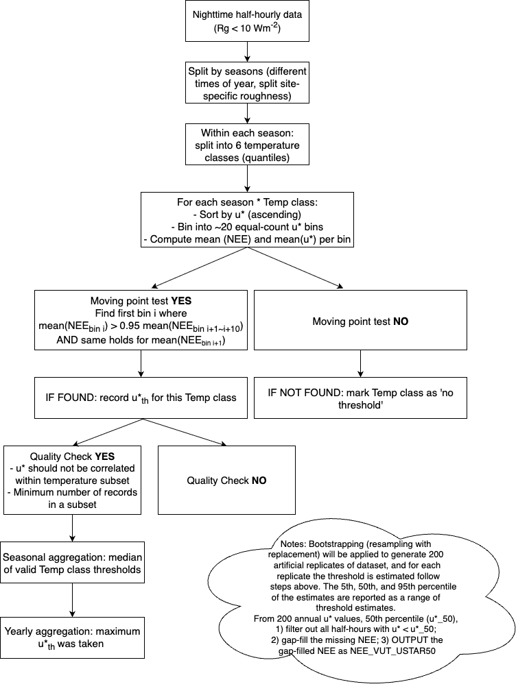
Scientists assumes a threshold of u* (detect the minimum amount of turbulence needed for reliable nighttime NEE (ecosystem respiration) measurements), two methods:
- The moving point method (Papale et al., 2006 https://doi.org/10.5194/bg-3-571-2006):
Seperate BINS: Only nighttime data used (Rg < 10 W m-2) -> seasonal splitting (data are split by seasons to account for changes in surface properties) -> temperature subsets (each season is further split into 6 temperature bins using quantiles, to ensure homogeneity of respiration rates, temperature is closely related to respiration rates!) -> within each temperature subset, u* is divided into ~20 bins with equal number of points
Moving Point Test: For each bin i, compute mean NEE of bin i (\(\mu_i\)) and mean NEE of the next 10 bins (\(\mu_{i+1\,\ldots\,i+10}\)) -> Check if \(\mu_i > 0.95 \times \operatorname{mean}(\mu_{i+1}, \ldots, \mu_{i+10})\) and this holds for \(\mu_{i+1}\)->If so, bin i’s mean u* is the threshold
Gap-filling
Look-up Tables (LUT)
Overview: Tables were created for each site so that missing values of FNEE could be “looked-up” based on environmental conditions associated with the missing data.
Pick a gap in the cleaned (QC + u* filtered) flux data (VAR_fall is NA).
Set the search window — user-defined WinDays.i days before and after the gap; full window length = 2 × WinDays.i days.
Choose condition variables and tolerances — up to 5 meteorological drivers (e.g., Rg ±50 W m⁻², Tair ±2.5 °C, VPD ±5 hPa).
- Special rule: If the first variable is Rg, reduce tolerance at low light to a minimum of 20 W m⁻² and never exceed the original tolerance, to avoid mismatching dark and bright conditions.
Find candidate records inside the time window that:
- Have a measured original value (VAR_orig not NA), and
- For each active driver, the absolute difference from the gap’s value is less than the set tolerance (using the adjusted Rg tolerance if applicable).
Check sample size: Require at least 2 valid matches to proceed.
Fill the gap:
- Value = mean of all matching records.
- Uncertainty = standard deviation (SD) of the matching records.
- fnum = number of matches used.
Assign method code and QC:
- fmeth = 1 if ≥3 drivers used; fmeth = 2 if only 1 driver used.
- QC = 1 for short windows (≤14 days full span for ≥3 drivers; ≤14 or ≤28 days for 1 driver), QC = 2 for medium windows, QC = 3 for long windows.
Write results back: Store filled value, number of matches, SD, method code, window length, and QC in VAR_fall and related columns. Only fill VAR_f if it’s still NA.
Skip if no fill: If <2 matches found, leave the gap for later methods (e.g., MDC) in the MDS cascade.
Mean Diurnal Course (MDC)
Overview: Fills missing flux values by averaging measurements from the same time of day (±1 hour) on nearby days, assuming that conditions at the same time of day are similar on days close together. Medium performance but it has advantage that this approach can be used even if no meteorological information is available.
Pick a gap in the cleaned (QC + u* filtered) flux data (VAR_fall is NA).
Set the search window — by default ±7 days around the gap (user-defined WinDays.i), giving a full window length of 2 × WinDays + 1 days.
Identify same-time-of-day neighbors:
Use the gap’s position in the day and collect indices for:
- The current day: ±2 records (≈±1 hour) around the gap time.
- Each day up to WinDays.i days before and after: same-time ±1 hour.
Keep only measured points: Remove any candidate records where the original flux (VAR_orig) is NA.
Check sample size: Require at least 2 valid neighbors to proceed.
Fill the gap:
- Value = mean of all valid neighbors.
- Uncertainty = standard deviation (SD) of those neighbors.
- fnum = number of neighbors used.
Assign method code and QC:
- fmeth = 3 (MDC method).
- fwin = number of days spanned (2 × WinDays + 1).
- QC = 1 if ≤1 day used; 2 if >1–5 days; 3 if >5 days.
Write results back: Store filled value, number of points, SD, method code, window length, and QC in VAR_fall and related columns. Only fill VAR_f if it’s still NA.
Marginal Distribution Sampling (MDS)
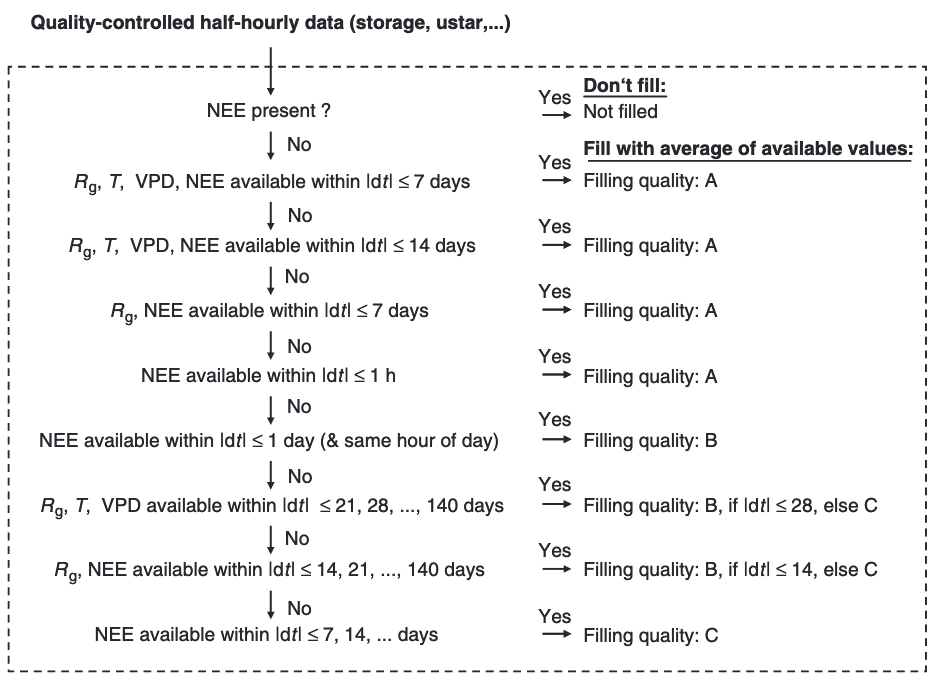
Overview: To solve the 1) covariation of the fluxes with the meteorological variables and 2) temporal autocorrelation based on LUT and MDC
(1) Only the data of direct interest are missing, but all meteorological data are available
-> [LUT] the missing value is replaced by the average value under similar meteorological conditions within a time-window of 7 days. Similar meteorological conditions are present when Rg, Tair and VPD do not deviate by more than 50 W m 2, 2.5 1C, and 5.0 hPa, respectively. If no similar meteorological conditions, averaging window is increased to 14 days.
(2) Air temperature or VPD is missing, but radiation is available
-> the same approach is taken, but similar meteorological conditions can only be defined via Rg deviation less than 50 W m 2
(3) Radiation data is missing
-> the missing value is replaced by the average value at the same time of the day (1 h), i.e. by the mean diurnal course. In this case, the window size starts with 0.5 days
For other gap filling methods and related evaluations, 10.1016/j.agrformet.2007.08.011